A Python ETL from Teradata to PostgreSQL with ADBC drivers and Polars

The Python ecosystem has a library for most things one can do with data. The data itself, however, is mostly stored in databases. To use these libraries, it has to leave the database, be processed in Python, and go back to a database, the same one or another, through the drivers in between.

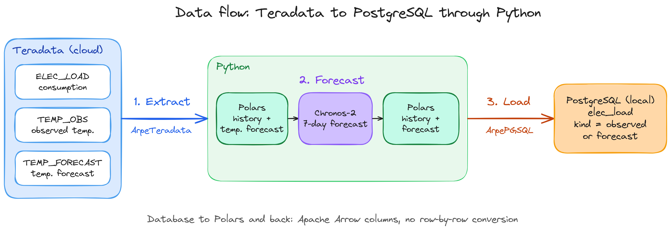
Here, we go through such a round trip in three steps: we extract the hourly electricity consumption of France and the temperature from Teradata into Polars DataFrames, forecast the next seven days with Chronos-2, a pretrained time series model, and load the history and the forecast into PostgreSQL. The forecast is only an example of processing done in between; the subject is the data movement.

The two databases are reached with our ADBC drivers, ArpeTeradata and ArpePGSQL, which speak the wire protocol of each database natively, without a vendor client library. ADBC drivers return and accept Apache Arrow data. The wire protocols of Teradata and PostgreSQL are row-based: when reading, the driver transposes the rows into Arrow columns, and when writing, it transposes the columns back into rows. A query result therefore arrives in the columnar format used by Polars, and a DataFrame is written without being converted to rows in Python. Our drivers are also optimized for speed at every level.

Data

Electricity consumption

The series is the national electricity consumption of mainland France, from the éCO2mix consolidated and definitive data published by RTE on the ODRÉ open data portal, under the Licence Ouverte v2.0.

These data come from meter readings. RTE publishes them as consolidated once checked and completed, usually around the middle of the following month, and as definitive once all partners have checked their readings, in the second half of the following year. When we downloaded them on November 6, 2026, they were definitive until December 2024, consolidated after that, and ended on August 31, 2026.

The consumption is given in MW every 30 minutes. We averaged it by hour, in UTC to avoid the daylight saving time changes, from January 1, 2012 to August 31, 2026, Paris time, which gives 128,567 rows. The 14 missing hours were filled by linear interpolation.

Temperature

Electricity consumption in France depends on the temperature, so the model also gets it. The hourly temperature comes from Open-Meteo, under the CC BY 4.0 licence, at 8 cities: Paris, Lyon, Marseille, Lille, Toulouse, Bordeaux, Nantes and Strasbourg. We averaged them, weighted by the approximate population of each urban area. RTE uses its own reference temperature, a weighted average over Météo-France stations; ours is a simpler substitute. There are two series:

• the observed temperature, from the ERA5 reanalysis, over the same hours as the consumption. It contains modified Copernicus Climate Change Service information;
• the temperature forecast for September 1 to 7, issued on August 31 at 21:00 UTC, from Open-Meteo's archive of previous model runs. An hour h hours ahead takes a model run started at least h hours earlier. A run is published a few hours after it starts, so a few of these hours may use a run that came out shortly after 21:00.

Météo-France publishes its hourly observations as open data, but we did not find an archive of its past forecasts over 7 days, hence Open-Meteo for both series.

Tables

All rows were loaded into a ClearScape Analytics Experience trial environment with ArpeTeradata's bulk ingest, cursor.adbc_ingest, from our machine over TLS. The driver created MULTISET NO PRIMARY INDEX tables. All timestamps are in UTC, stored without time zone:

table	columns	rows
ELEC_LOAD	ts TIMESTAMP(3), load_mw INTEGER	128,567
TEMP_OBS	ts TIMESTAMP(3), temp_c FLOAT	128,590
TEMP_FORECAST	issued TIMESTAMP(3), ts TIMESTAMP(3), temp_c FLOAT	168

The result goes to a PostgreSQL database, energy, running locally in Docker.

Setup

Each driver is installed and registered with the ADBC driver manager by a one-line script, as described in the documentation. The script takes the path of a licence file. You can get a free 30-day trial licence for ArpeTeradata and for ArpePGSQL from the trial page, which also gives the install command:

curl -fsSL https://raw.githubusercontent.com/arpe-io/adbc-drivers/main/install.sh \
  | sh -s -- arpeteradata --license /path/to/your.lic
curl -fsSL https://raw.githubusercontent.com/arpe-io/adbc-drivers/main/install.sh \
  | sh -s -- arpepgsql --license /path/to/your.lic

On the Python side, chronos-forecasting brings PyTorch and pandas:

pip install adbc-driver-manager polars pyarrow chronos-forecasting

System and package versions

Python               : 3.14.2
OS                   : Linux
adbc_driver_manager  : 1.13.0
polars               : 2.1.0
pyarrow              : 26.0.1
chronos-forecasting  : 2.3.2
torch                : 2.14.1
pandas               : 2.3.3
ArpeTeradata         : 0.3.6
ArpePGSQL            : 0.4.9
Teradata             : 20.00.24.60 (ClearScape Analytics Experience)
PostgreSQL           : 17.6

Imports

import adbc_driver_manager.dbapi as dbapi
import polars as pl
from chronos import Chronos2Pipeline

Step 1: Extract from Teradata

The default sslmode is prefer, which falls back to an unencrypted connection on port 1025 if the TLS logon fails; with require, the connection uses TLS on port 443 or fails. A password with special characters has to be percent-encoded in the URI, for example with urllib.parse.quote(password, safe="").

The first query joins the consumption and the observed temperature in Teradata, the second one reads the latest temperature forecast, the one issued on August 31:

td_uri = "teradata://demo_user:<password>@<host>?sslmode=require"

with dbapi.connect(driver="arpeteradata", db_kwargs={"uri": td_uri}) as conn:
    load = pl.read_database(
        "SELECT l.ts, l.load_mw, t.temp_c "
        "FROM ELEC_LOAD l JOIN TEMP_OBS t ON t.ts = l.ts ORDER BY l.ts",
        conn,
    )
    temp_fc = pl.read_database(
        "SELECT issued, ts, temp_c FROM TEMP_FORECAST "
        "WHERE issued = (SELECT MAX(issued) FROM TEMP_FORECAST) ORDER BY ts",
        conn,
    )

The 128,567 + 168 rows arrive in 3.06 s, connection included. This time is limited by the network: the ClearScape environment runs in the cloud, and the client is a laptop on Wi-Fi. The join keeps all the 128,567 hours of ELEC_LOAD: an hour without temperature would have been dropped silently. TIMESTAMP is mapped to Datetime, INTEGER to Int32 and FLOAT to Float64. Chronos-2 uses at most the last 8,192 hours as context, about 11 months, so a WHERE clause could reduce the transfer; we read the whole history to move a larger volume.

load.tail(3)

shape: (3, 3)
┌─────────────────────┬─────────┬────────┐
│ ts                  ┆ load_mw ┆ temp_c │
│ ---                 ┆ ---     ┆ ---    │
│ datetime[μs]        ┆ i32     ┆ f64    │
╞═════════════════════╪═════════╪════════╡
│ 2026-08-31 19:00:00 ┆ 46421   ┆ 20.52  │
│ 2026-08-31 20:00:00 ┆ 44598   ┆ 19.97  │
│ 2026-08-31 21:00:00 ┆ 44524   ┆ 19.52  │
└─────────────────────┴─────────┴────────┘

temp_fc.head(3)

shape: (3, 3)
┌─────────────────────┬─────────────────────┬────────┐
│ issued              ┆ ts                  ┆ temp_c │
│ ---                 ┆ ---                 ┆ ---    │
│ datetime[μs]        ┆ datetime[μs]        ┆ f64    │
╞═════════════════════╪═════════════════════╪════════╡
│ 2026-08-31 21:00:00 ┆ 2026-08-31 22:00:00 ┆ 20.02  │
│ 2026-08-31 21:00:00 ┆ 2026-08-31 23:00:00 ┆ 19.51  │
│ 2026-08-31 21:00:00 ┆ 2026-09-01 00:00:00 ┆ 18.78  │
└─────────────────────┴─────────────────────┴────────┘

Step 2: Forecast with Chronos-2

Chronos-2 is a transformer model with 120 million parameters, pretrained by Amazon on real and synthetic time series. It forecasts a new series without being trained on it: we give it the history and the number of steps, 168 hours, and it returns quantiles of the forecast. The 5% and 95% quantiles bound a 90% prediction interval.

The temperature is passed as a covariate: its past values come with the history, and its future values, the forecast issued on August 31, in future_df. The weights, 478 MB, are downloaded from Hugging Face on the first call, and the model runs on the CPU.

predict_df takes pandas DataFrames with an identifier column, so the Polars DataFrames are converted with to_pandas(), and the result back with pl.from_pandas(). The forecast temperature and its issue date are joined to the result:

pipeline = Chronos2Pipeline.from_pretrained("amazon/chronos-2", device_map="cpu")
pred = pipeline.predict_df(
    load.with_columns(id=pl.lit("FR")).to_pandas(),
    future_df=temp_fc.drop("issued").with_columns(id=pl.lit("FR")).to_pandas(),
    id_column="id",
    timestamp_column="ts",
    target="load_mw",
    prediction_length=168,
    quantile_levels=[0.05, 0.5, 0.95],
)
forecast = pl.from_pandas(pred).select(
    pl.col("ts").dt.cast_time_unit("us"),
    pl.col("0.5").round().cast(pl.Int32).alias("load_mw"),
    pl.col("0.05").round().cast(pl.Int32).alias("load_mw_lo90"),
    pl.col("0.95").round().cast(pl.Int32).alias("load_mw_hi90"),
).join(temp_fc, on="ts")
forecast.drop("issued", "temp_c").head(3)

shape: (3, 4)
┌─────────────────────┬─────────┬──────────────┬──────────────┐
│ ts                  ┆ load_mw ┆ load_mw_lo90 ┆ load_mw_hi90 │
│ ---                 ┆ ---     ┆ ---          ┆ ---          │
│ datetime[μs]        ┆ i32     ┆ i32          ┆ i32          │
╞═════════════════════╪═════════╪══════════════╪══════════════╡
│ 2026-08-31 22:00:00 ┆ 42415   ┆ 41677        ┆ 43071        │
│ 2026-08-31 23:00:00 ┆ 39852   ┆ 39188        ┆ 40522        │
│ 2026-09-01 00:00:00 ┆ 38107   ┆ 37253        ┆ 38733        │
└─────────────────────┴─────────┴──────────────┴──────────────┘

Loading the model and forecasting take 1.35 s, with the weights already downloaded. The forecast starts at the hour following the last row in Teradata, August 31 at 22:00 UTC, which is midnight on September 1 in Paris, and ends on September 7 at 21:00 UTC.

load_mw is the median forecast. load_mw_lo90 and load_mw_hi90 are the bounds of the 90% prediction interval: if the model is well calibrated, the actual consumption should fall between them in 90% of the hours. The interval widens with the horizon: 1.4 GW wide for the first hour, 2.6 GW after one day, and 6.7 GW for the last hour.

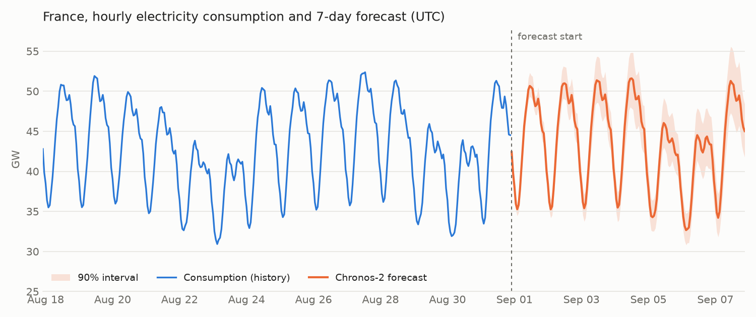
The last two weeks of history and the forecast for September 1 to 7, 2026.

Step 3: Load into PostgreSQL

The history and the forecast go into a single table, elec_load. The kind column tells them apart, observed or forecast. issued is the issue date of the forecast, so that several forecasts can be kept in the table; it is null for the observed rows, as are the interval bounds. The timestamps are marked as UTC so that PostgreSQL stores them with their time zone:

elec = pl.concat(
    [
        load.with_columns(kind=pl.lit("observed")),
        forecast.with_columns(kind=pl.lit("forecast")),
    ],
    how="diagonal",
).select(
    pl.col("ts").dt.replace_time_zone("UTC"),
    "kind",
    pl.col("issued").dt.replace_time_zone("UTC"),
    "load_mw", "load_mw_lo90", "load_mw_hi90", "temp_c",
)
elec.select("ts", "kind", "load_mw", "temp_c").tail(3)

shape: (3, 4)
┌─────────────────────────┬──────────┬─────────┬────────┐
│ ts                      ┆ kind     ┆ load_mw ┆ temp_c │
│ ---                     ┆ ---      ┆ ---     ┆ ---    │
│ datetime[μs, UTC]       ┆ str      ┆ i32     ┆ f64    │
╞═════════════════════════╪══════════╪═════════╪════════╡
│ 2026-09-07 19:00:00 UTC ┆ forecast ┆ 46496   ┆ 23.44  │
│ 2026-09-07 20:00:00 UTC ┆ forecast ┆ 45520   ┆ 22.43  │
│ 2026-09-07 21:00:00 UTC ┆ forecast ┆ 45025   ┆ 21.29  │
└─────────────────────────┴──────────┴─────────┴────────┘

write_database with engine="adbc" accepts the ADBC connection and sends the DataFrame through ArpePGSQL's bulk ingest, which creates the table. The local container has no TLS, hence sslmode=disable:

pg_uri = "postgresql://postgres:<password>@localhost:5434/energy?sslmode=disable"

with dbapi.connect(driver="arpepgsql", db_kwargs={"uri": pg_uri}) as conn:
    elec.write_database(
        "elec_load", conn, engine="adbc", if_table_exists="replace"
    )

The 128,735 rows are written in 0.08 s, connection included. The table has two timestamp with time zone columns, a text column, three integer columns and a double precision column. if_table_exists="replace" drops and recreates the table at each run; a scheduled job would rather append the rows of each new forecast, told apart by issued, and the new observed hours.

We read back the number of rows by kind and issue date, and the rows around the forecast start. The wider outputs are shown with a selection of columns:

with dbapi.connect(driver="arpepgsql", db_kwargs={"uri": pg_uri}) as conn:
    check = pl.read_database(
        "SELECT kind, issued, COUNT(*) AS n "
        "FROM elec_load GROUP BY kind, issued ORDER BY kind DESC",
        conn,
    )
    start = pl.read_database(
        "SELECT ts, kind, load_mw, temp_c FROM elec_load "
        "WHERE ts BETWEEN '2026-08-31 20:00+00' AND '2026-08-31 23:00+00' "
        "ORDER BY ts",
        conn,
    )
check

shape: (2, 3)
┌──────────┬─────────────────────────┬────────┐
│ kind     ┆ issued                  ┆ n      │
│ ---      ┆ ---                     ┆ ---    │
│ str      ┆ datetime[μs, UTC]       ┆ i64    │
╞══════════╪═════════════════════════╪════════╡
│ observed ┆ null                    ┆ 128567 │
│ forecast ┆ 2026-08-31 21:00:00 UTC ┆ 168    │
└──────────┴─────────────────────────┴────────┘

start

shape: (4, 4)
┌─────────────────────────┬──────────┬─────────┬────────┐
│ ts                      ┆ kind     ┆ load_mw ┆ temp_c │
│ ---                     ┆ ---      ┆ ---     ┆ ---    │
│ datetime[μs, UTC]       ┆ str      ┆ i32     ┆ f64    │
╞═════════════════════════╪══════════╪═════════╪════════╡
│ 2026-08-31 20:00:00 UTC ┆ observed ┆ 44598   ┆ 19.97  │
│ 2026-08-31 21:00:00 UTC ┆ observed ┆ 44524   ┆ 19.52  │
│ 2026-08-31 22:00:00 UTC ┆ forecast ┆ 42415   ┆ 20.02  │
│ 2026-08-31 23:00:00 UTC ┆ forecast ┆ 39852   ┆ 19.51  │
└─────────────────────────┴──────────┴─────────┴────────┘

Results

The consolidated data stop on August 31, so the model never saw the forecast week, which is now in the past. Chronos-2 was released in October 2025, so none of the weeks scored here can be in its training data.

The consumption of that week is available in a second RTE dataset on the same portal and under the same licence, the éCO2mix real-time data. These are telemetry data from the grid, completed with estimates, at a 15-minute step and refreshed every 15 minutes. RTE removes each month from this dataset once it is consolidated, so the real-time data start where the consolidated data end, on August 31 at 22:00 UTC. They have not been checked yet and may differ slightly from the future consolidated values.

We took the actual consumption for the 168 forecast hours from it, averaged by hour in the same way, only to score the forecast. These data were not loaded into Teradata or given to the model.

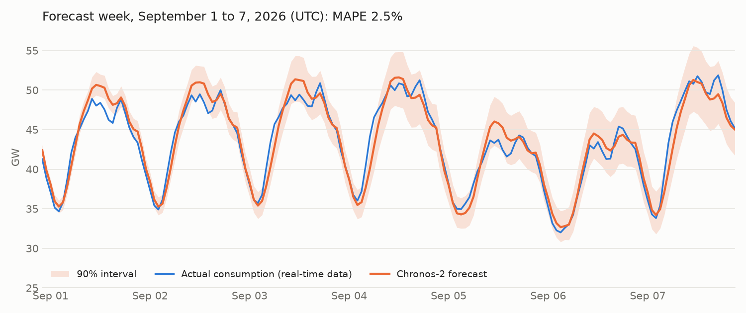
The forecast week alone, with the actual consumption from the éCO2mix real-time data.

The mean absolute percentage error (MAPE) over the 168 hours is 2.46%. 141 of the 168 actual values (84%) fall inside the 90% interval, and 14 of the 27 misses are on September 1: the interval is too narrow for the first hours.

In a backtest over the 8 previous weeks, each forecast with the temperature forecast available at its date and scored against the consolidated data, the temperature reduced the MAPE of Chronos-2 from 2.7% to 2.2%, and 95% of the values fall inside the 90% interval. These are summer weeks; in winter, with electric heating, the consumption depends more on the temperature.

The forecast is a reconstruction: on August 31, the consolidated consumption of the last days of August and their ERA5 temperatures were not published yet. In operation, these hours would come from the real-time consumption data and from weather station observations.

Reading from Teradata, forecasting and writing to PostgreSQL took 4.5 s, most of it spent reading the 128,567 rows from the cloud. This dataset is small; the benefit of columnar, optimized drivers grows with the volume of data.

Driver downloads are at github.com/arpe-io/adbc-drivers. The binaries download freely and run once a licence is present. A 30-day trial licence can be downloaded for free for ArpeTeradata and ArpePGSQL; for a full licence, contact us at sales@arpe.io or see arpe.io.

Try ArpeTeradata Now Try ArpePGSQL Now

Free 30-day trial